Parameter inversion

Assume a dynamical system $f$ generates an output $y$ based on its input $x$ and on a set of parameters $\theta$. The goal of a parameter inversion is to estimate the parameters $\theta$ that best fit the data $\hat{y}$ with respect to an error metric $\Psi$, i.e. to solve the following optimization problem:

\[\begin{aligned} y &=& f(x, \theta) \\ \hat{\theta} &=& \arg\min_{\theta} \Psi(\hat{y} - y) \end{aligned}\]

Since FastIsostasy relies on simplifications of the full GIA problem, applying such inversion can be useful to tune the model parameters (upper-mantle viscosity field, lithospheric thickness... etc.) such that the output $y$ (typically the displacement) matches the data $\hat{y}$ (typically obtained from observations or from a 3D GIA model). There are many ways of solving this problem, among which the use of Kalman filtering techniques. FastIsostasy.jl provides convenience functions for the latter by wrapping the functionalities of EnsembleKalmanProcesses.jl in an external routine that is automatically loaded when using EnsembleKalmanProcesses.

We demonstrate the tuning of the effective viscosity in a region that is being forced by a circular ice load. We emphasise that the highlighted tools provided by FastIsostasy are not limited to this case. As it will be made clear throughout the example, the user merely needs to define their own ParameterReduction and the associated behaviours of reconstruct! and extract_output to adapt the inversion procedure to their needs (e.g. tune lithospheric thickness throughout the whole domain).

We first load the necessary packages, initialize the ComputationDomain and assign laterally-variable viscosity profiles to a LayeredEarth by loading the fields estimated in Wiens et al. (2022):

using CairoMakie
using Distributions
using EnsembleKalmanProcesses
using EnsembleKalmanProcesses.ParameterDistributions
using FastIsostasy
using LinearAlgebra

Omega = ComputationDomain(3000e3, 5)
c = PhysicalConstants()
lb = [100e3, 200e3, 300e3]
_, eta, eta_itp = load_dataset("Wiens2022")
loglv = cat([eta_itp.(Omega.X, Omega.Y, z) for z in lb]..., dims = 3)
lv = 10 .^ loglv
p = LayeredEarth(Omega, layer_boundaries = lb, layer_viscosities = lv)

LayeredEarth{Float64, Matrix{Float64}}([2.8882687455337736e20 8.390101128670159e20 … 7.11238760892716e20 2.548861742533004e20; 4.9859163933404686e20 2.8563286881831748e20 … 6.124735899366491e20 2.145763590353581e20; … ; 7.842816921212305e20 8.112869530785191e20 … 7.118861791640621e20 6.685915619309133e20; 5.342589933662746e20 7.656245072962721e20 … 3.080940856185763e20 3.5344830301378085e20], [100000.0 100000.0 … 100000.0 100000.0; 100000.0 100000.0 … 100000.0 100000.0; … ; 100000.0 100000.0 … 100000.0 100000.0; 100000.0 100000.0 … 100000.0 100000.0], [5.967881944444444e24 5.967881944444444e24 … 5.967881944444444e24 5.967881944444444e24; 5.967881944444444e24 5.967881944444444e24 … 5.967881944444444e24 5.967881944444444e24; … ; 5.967881944444444e24 5.967881944444444e24 … 5.967881944444444e24 5.967881944444444e24; 5.967881944444444e24 5.967881944444444e24 … 5.967881944444444e24 5.967881944444444e24], 0.28, 0.28, [2.6981748e10 2.6981748e10 … 2.6981748e10 2.6981748e10; 2.6981748e10 2.6981748e10 … 2.6981748e10 2.6981748e10; … ; 2.6981748e10 2.6981748e10 … 2.6981748e10 2.6981748e10; 2.6981748e10 2.6981748e10 … 2.6981748e10 2.6981748e10], 6.6e10, 2.578125e10, 3400.0, 3200.0)

To make this problem more exciting, we place the center of the ice load to $(-1000, -1000) \: \mathrm{km}$ where the viscosity field displays a less uniform structure. For the sake of simplicity, the data to fit is obtained from a FastIsostasy simulation with the ground-truth viscosity field.

R, H = 1000e3, 1e3
Hcylinder = uniform_ice_cylinder(Omega, R, H, center = [-1000e3, -1000e3])
Hice = [zeros(Omega.Nx, Omega.Ny), Hcylinder, Hcylinder]
t_out = collect(1e3:1e3:2e3)
pushfirst!(t_out, t_out[1]-1e-8)
t_Hice = copy(t_out)

true_viscosity = copy(p.effective_viscosity)
fip = FastIsoProblem(Omega, c, p, t_out, t_Hice, Hice, output = "sparse")
solve!(fip)

Assuming the result of this simulation to be the ground truth $\hat{y}$, we can now build an InversionData object that will be passed to an InversionProblem. The InversionData object contains the time series of the input field X = Hice and the output field Y = extract_fip(fip) (here the displacement field). Furthermore, we define an InversionConfig that uses the unscented Kalman filter as introduced in Huang and Huang (Feb 2021).

X = Hice
mask3D = cat([x .> 0 for x in X]..., dims = 3)
mask = reduce(|, mask3D, dims = 3)[:, :, 1]     # Only tune viscosity where there is ice.

t_inv = t_out[end:end]                          # Only use last time step for inversion.
extract_last_viscous_displacement(fip) = fip.out.u[end:end]
extract_fip = extract_last_viscous_displacement
Y = extract_fip(fip)

data = InversionData(t_inv, length(t_inv), X, Y, mask, count(mask))
config = InversionConfig(Unscented, N_iter = 15, scale_obscov = 10.0)

InversionConfig{Float64}(EnsembleKalmanProcesses.Unscented, 15, 1.0, 1, 100, 10.0)

Before finalising the inversion, we need to specify a ParameterReduction, which allows a multiple dispatch of reconstruct!, extract_output and (optionally) print_inversion_evolution. This allows the inversion procedure to update the parameters, extract the relevant output and (optionally) print out meaningful information over the iterations of the inversion procedure. In this example, we define a ViscosityRegion that reduces the number of parameters to the number of grid points in the mask.

struct ViscosityRegion{T<:AbstractFloat} <: ParameterReduction{T}
    mask::BitMatrix
    nparams::Int
end

function FastIsostasy.reconstruct!(fip, params, reduction::ViscosityRegion)
    fip.p.effective_viscosity[reduction.mask] .= 10 .^ params
end

function FastIsostasy.extract_output(fip, reduction::ViscosityRegion, data::InversionData)
    return extract_fip(fip)[1][reduction.mask]
end

function FastIsostasy.print_inversion_evolution(paraminv, n, ϕ_n, reduction::ViscosityRegion)
    err_n = paraminv.error[n]
    cov_n = paraminv.ukiobj.process.uu_cov[n]

    println("-----------------------------------------------------")
    println("Inversion being performed with $(typeof(reduction)) as a parameter reduction")
    @show size(ϕ_n), n, err_n, norm(cov_n)
    println("Mean tuned log10-viscosity: $(round(mean(ϕ_n), digits = 3))")
    println("Extrema of tuned log10-viscosity: $(extrema(ϕ_n))")
    return nothing
end

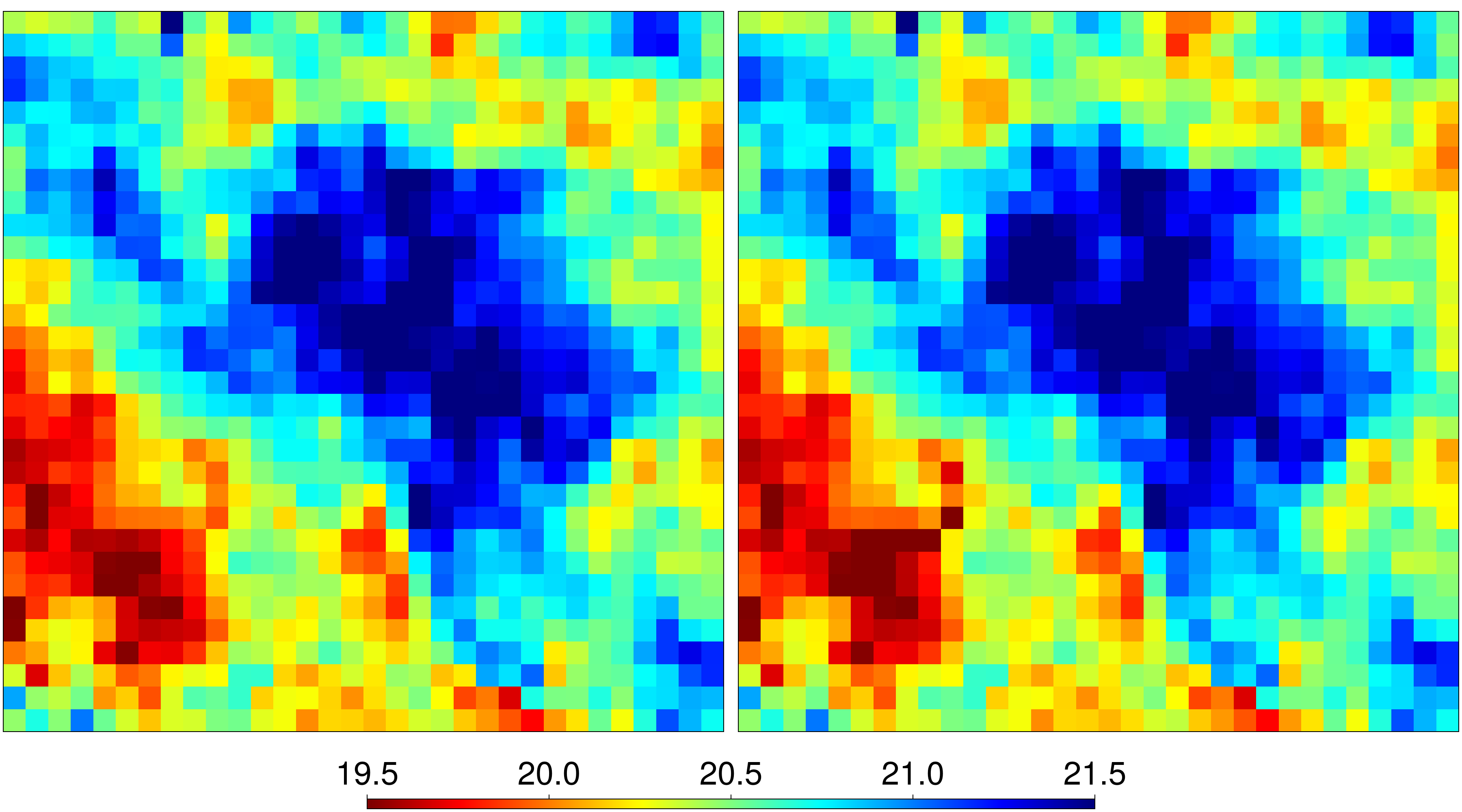
reduction = ViscosityRegion{Float64}(mask, count(mask))

Main.ViscosityRegion{Float64}(Bool[0 0 … 0 0; 0 0 … 0 0; … ; 0 0 … 0 0; 0 0 … 0 0], 86)

We can now proceed to the definition of the InversionProblem with a prior distribution that is a Gaussian with mean $20.5$, variance $0.5$ and bounds $[19.0, 22.0]$. We then check the initialisation of the inversion problem by reconstructing the field with the prior parameters:

priors = combine_distributions([constrained_gaussian( "p_$(i)",
    20.5, 0.5, 19.0, 22.0) for i in 1:reduction.nparams])
paraminv = inversion_problem(deepcopy(fip), config, data, reduction, priors)

params = fill(20.5, count(mask))
reconstruct!(paraminv.fip, params, reduction)
function plot_viscfields(paraminv)
    cmap = cgrad(:jet, rev = true)
    crange = (19.5, 21.5)
    fig = Figure(size = (1800, 1000), fontsize = 40)
    axs = [Axis(fig[1,i], aspect = DataAspect()) for i in 1:2]
    [hidedecorations!(ax) for ax in axs]
    heatmap!(axs[1], log10.(true_viscosity), colormap = cmap, colorrange = crange)
    heatmap!(axs[2], log10.(paraminv.fip.p.effective_viscosity),
        colormap = cmap, colorrange = crange)
    Colorbar(fig[2, :], vertical = false, colormap = cmap, colorrange = crange,
        width = Relative(0.5))
    return fig
end
fig1 = plot_viscfields(paraminv)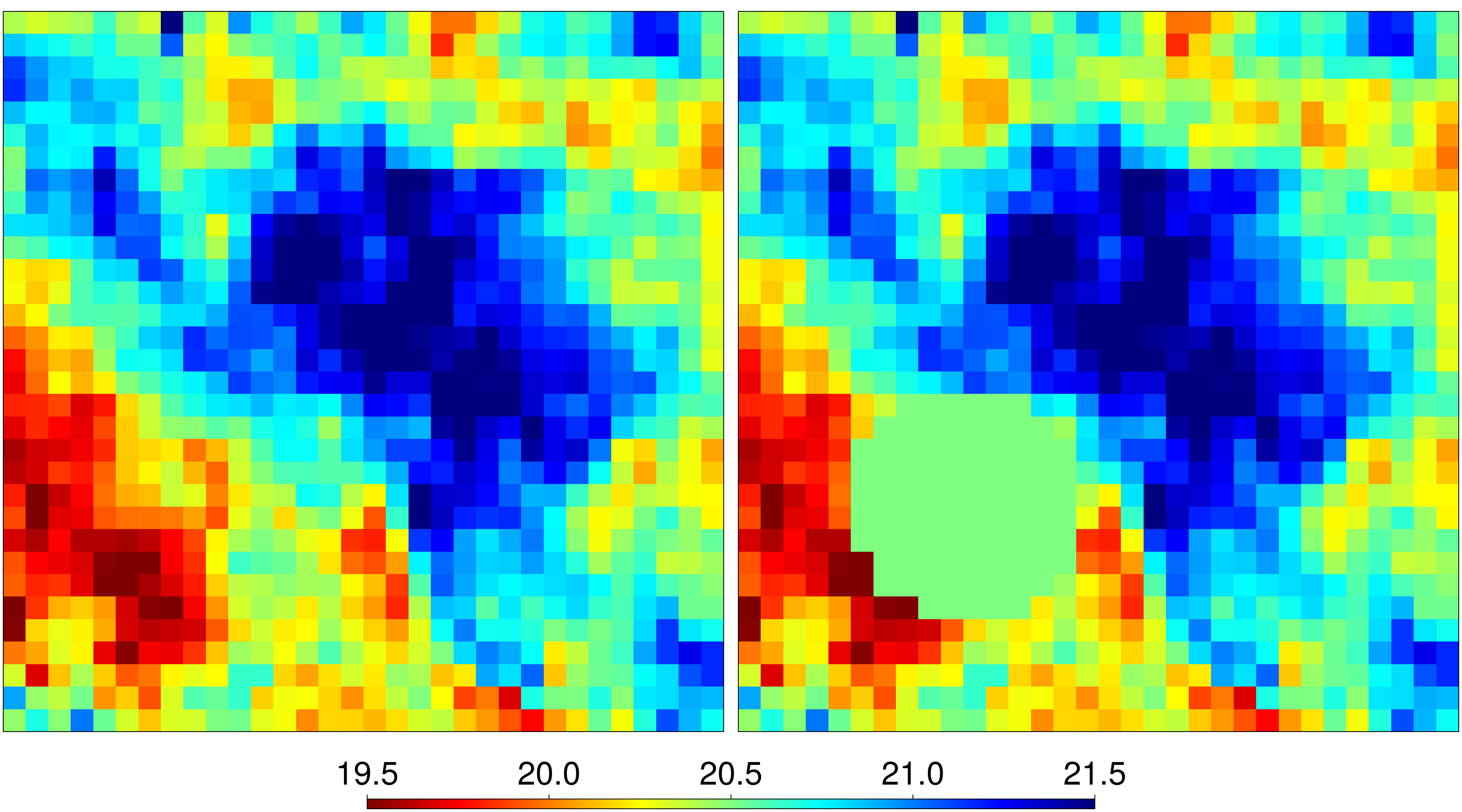

Finally, we solve the inversion problem and visualise the results.

solve!(paraminv)
fig2 = plot_viscfields(paraminv)