Analytical benchmark
We here present a simple example to benchmark the accuracy of the numerical scheme against an analytical solution. The setup is the same as in Bueler et al. (2007), where a cylindrical ice load with a radius of $1000 \, \mathrm{km}$ and a thickness of $1 \, \mathrm{km}$ is applied to a laterally homogeneous Maxwell body. First, let's generate the load and the computation domain:
using FastIsostasy, CairoMakie

W, n = 3f6, 7   # square domain with size 2*W and 2^n points in each dimension
domain = RegionalDomain(W, n)

H_ice_0 = zeros(domain)             # Load: 0 at the beginning...
H_ice_1 = 1f3 .* (domain.R .< 1f6)  # cylinder afterwards
fig = plot_load(domain, H_ice_1)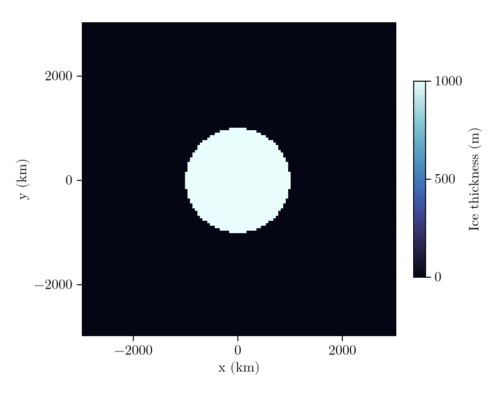
This looks as expected. plot_load is a function of FastIsostasy that, similar to all functions plot_*, is only loaded if the user is using Makie. These functions are here quickly visualize results and are summarized in the API reference.
In the next step, we wrap the ice load as a time interpolator so that the boundary conditions of FastIsostasy can be updated internally (if you want to update the ice thickness externally, have a look at this). We then define a solid earth structure, a sea-level model (that is inactive by default) and an output object. The Earth structure deserves particular attention, since it determines key properties of the problem. We here define a lithosphere with thickness $T = 88 \, \mathrm{km}$ and an upper-mantle with viscosity $\eta = 10^{21} \, \mathrm{Pa \, s}$. This results in a laterally homogeneous Maxwell body, which is a standard choice in simplified GIA modelling. For now, the lithosphere is assumed to be rigid in order to easily compare the results to the analytical solution of the viscous displacement.
t_ice = [0, 1, 50f3]
H_ice = [H_ice_0, H_ice_1, H_ice_1]
it = TimeInterpolatedIceThickness(t_ice, H_ice, domain)
bcs = BoundaryConditions(domain, ice_thickness = it)

solidearth = SolidEarth(                    # same geometry as Bueler et al. (2007).
    domain,
    rho_litho = 0f0,
    layer_boundaries = [88f3],
    layer_viscosities = [1f21],
)

sealevel = RegionalSeaLevel()               # default: inactive.

nout = NativeOutput(vars = [:u],            # only store viscous displacement.
    t = [100, 500, 1500, 5000, 10_000, 50_000f0]);
Explicit time stepping (recommended)
The default time stepping is explicit and adaptive, which is recommended for most applications. For more information on the time stepping, please refer to the API reference and the Integrators section. We now have all ingredients to create a simulation object and run the simulation:
sim = Simulation(domain, bcs, sealevel, solidearth, (0, 50f3); nout = nout)
run!(sim)
fig = plot_transect(sim, [:u])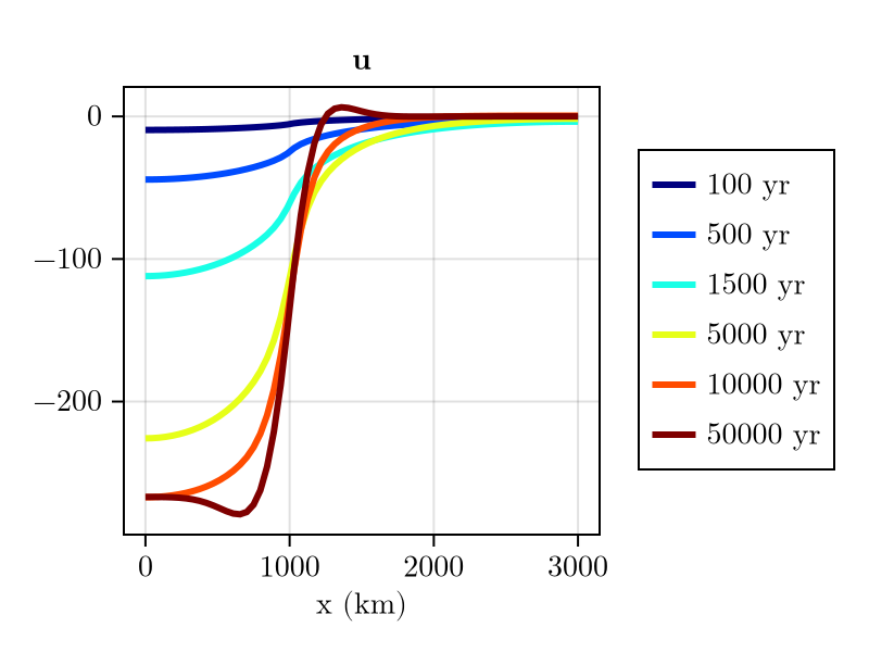
The viscous displacement field that we obtained is quite intuitive: its shape is largely determined by the forcing and its maximal amplitude is a fraction of the ice thickness is about $\dfrac{ \rho_\mathrm{ice} }{ \rho_\mathrm{mantle} }$. This simple example presents the advantage of having an analytical solution, which can be plotted along our solution:
fig = plot_transect(sim, [:u], analytic_cylinder_solution = true)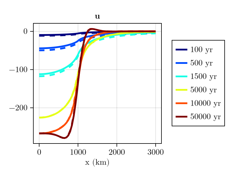
This confirms that our numerical scheme accurately reproduces the analytical solution! Furthermore, FastIsostasy was designed to be computationally efficient. We are therefore particularly interested in the time needed for the computation, which is stored as a vector sim.timer.t_computation:
fig, ax, _ = lines(sim.timer.t_computation, sim.timer.t_vec, label = "Explicit")
ax.xlabel = "Computation time (s)"
ax.ylabel = "Simulation years"
fig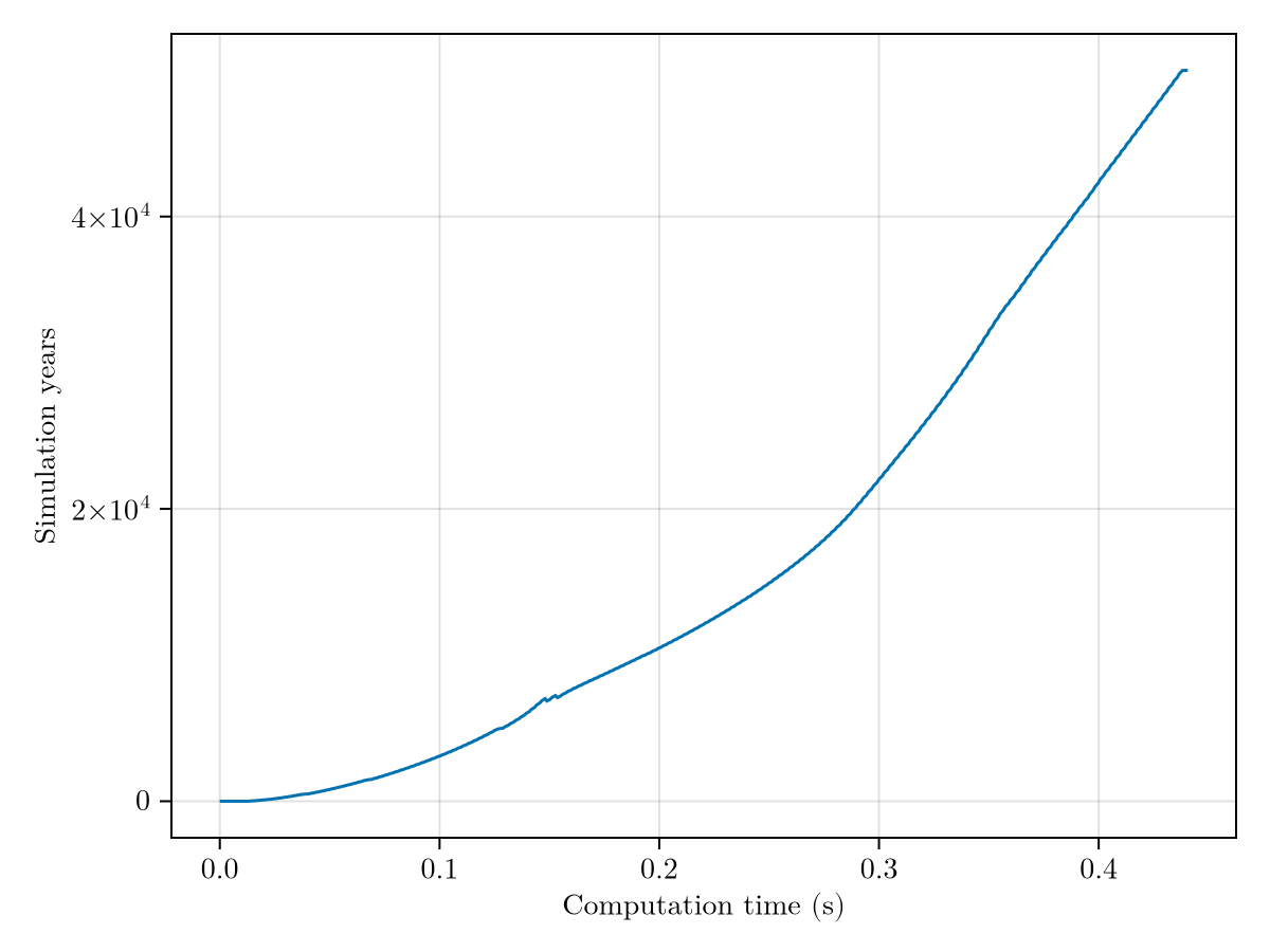
Yes, this is the computation time that was required to compute $50 \, \mathrm{kyr}$ of viscous displacement with a domain of 128x128 points! Pretty fast, huh?
Implicit time stepping
If the Earth structure is laterally constant (i.e. the lithospheric thickness and the mantle viscosity do not vary in x and y), the performance can be improved by using an implicit time stepping, as derived by Bueler et al. (2007). This can be achieved by specifying the lithosphere as RigidLithosphere or as LaterallyConstantLithosphere and requires to set a fixed time step via EulerIntegrator in SolverOptions:
solidearth = SolidEarth(                    # same geometry as Bueler et al. (2007).
    domain,
    lithosphere = RigidLithosphere(),
    layer_boundaries = [88f3],
    layer_viscosities = [1f21],
)
opts = SolverOptions(integ = EulerIntegrator(dt = 100f0))
sim_implicit = Simulation(domain, bcs, sealevel, solidearth, (0, 50f3); nout = nout, opts = opts)
run!(sim_implicit)
fig_implicit = plot_transect(sim_implicit, [:u], analytic_cylinder_solution = true)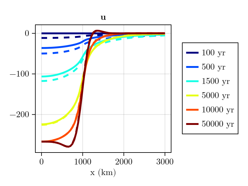
The results appear to be comparable with the previously obtained ones! However, the computation time is lower:
lines!(ax, sim_implicit.timer.t_computation, sim_implicit.timer.t_vec, label = "Implicit")
axislegend(ax, position = :lt)
fig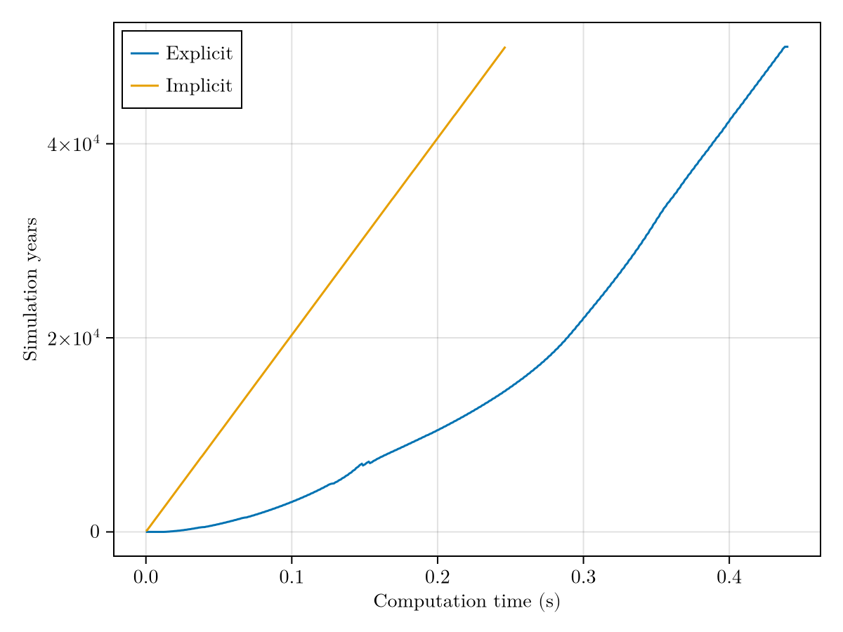
If you are not sure whether your Earth structure is laterally constant, you should not use the implicit time stepping. The results will be wrong if the lithosphere thickness or the mantle viscosity vary in x and y. Also, stability does not guarantee accuracy! In the present example, the time step of $100 \, \mathrm{yr}$ is not small enough to accurately resolve the initial phase of the viscous response. The implicit time stepping is therefore not recommended for general applications, but it can be used to speed up computations in very specific cases.
Floating-point precision
All of the computations shown above are performed with Float32 as floating point precision. It is easy to switch to Float64, by passing arguments as such (e.g. W = 3e6). This will increase the accuracy of the results, but also the computation time. The default Float32 is sufficient for most applications.
Of course, this example remains simple. If you want to learn how to increase the complexity of your simulations, go to the next examples!
Copy-pastable code
using FastIsostasy, CairoMakie

W, n = 3f6, 7                                # 6000 km box, 128 x 128
domain = RegionalDomain(W, n)

H_ice_1 = 1f3 .* (domain.R .< 1f6)           # 1 km thick, 1000 km radius cylinder
it = TimeInterpolatedIceThickness([0, 1, 50f3],
    [zeros(domain), H_ice_1, H_ice_1], domain)
bcs = BoundaryConditions(domain, ice_thickness = it)

solidearth = SolidEarth(domain, rho_litho = 0f0,
    layer_boundaries = [88f3], layer_viscosities = [1f21])
nout = NativeOutput(vars = [:u], t = [100, 500, 1500, 5000, 10_000, 50_000f0])

sim = Simulation(domain, bcs, RegionalSeaLevel(), solidearth, (0, 50f3); nout = nout)
run!(sim)

plot_transect(sim, [:u], analytic_cylinder_solution = true)